Handling large datasets in ArcGIS can be a truly painful process. When you are up against a deadline, the seconds spent wasted waiting for ArcGIS to update its display or run a query can be excruciating.
That is until you discover spatial indices! It is like a new world, where querying data is (almost) fun, and not an reason to go and make a cup of tea. Plus it is incredibly simple.
To apply a spatial index, firstly find your troublesome dataset in Catalog. Right-click and go to Properties. Then the Indexes tab. See Spatial Index in the bottom pane of this window and click Add. This will take a few seconds but once in place it will significantly improve the speed of your redrawing and querying.
Having said all this, I’m not sure this will be new to many – but I found this very useful. More information is available from ESRI themselves here.
At the very broadest scope, Space Syntax can be said to investigate the relationship between movement and the configuration and connectivity of space. In the past, while much favour has been found in the approach, critics have been distrustful of the axial line concept and of the representation of road segments as nodes in a network. The construction of the network too, the process of drawing a network of longest lines of sight, has been seen to be unscientific. Although I personally feel this to be a weak argument against Space Syntax in general, it’s acceptance into the wider research community may be hampered by this fact.
By way of a response to this argument, either intentionally or otherwise, there has been a movement towards segment-to-segment angularity (known as Angular Choice) as a predictor of movement. The method is described by Turner in this paper, but in summary it is a calculation of betweenness on each network segment using the angular deviation between segments as the weight on which to calculate a shortest path. The higher scoring segments, therefore, are those which are on a larger number of shortest angular paths passing over them.
One implication of this approach is that it a better fit for through-movement, that is an indicator of the routes we’re likely to use when moving from A to B. This fits with what has been identified in other literature (particularly spatial cognition) where least angular change is identified as a driver of choice, notably in favour of pure metric distance.
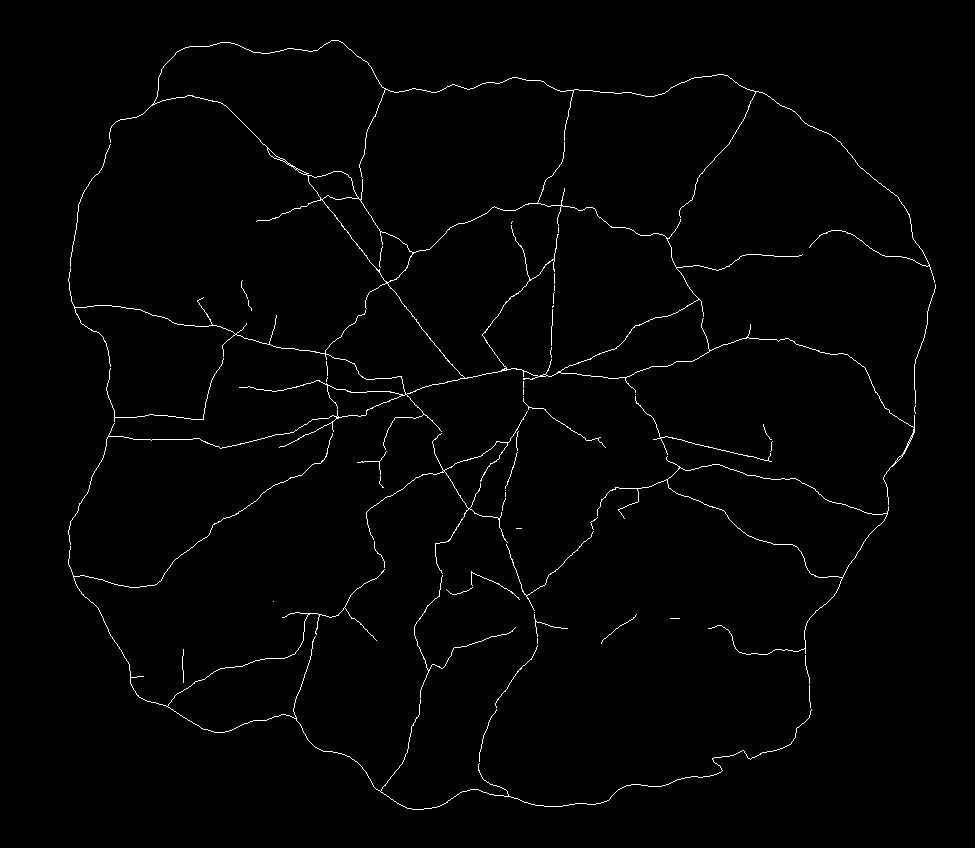
So with a view to better understanding this relationship between the reality and angular choice, I wanted to compare the networks we find in the city and those indicated by this measure. The first step was to draw out what traffic planners view as the most important roads on the network. These are the roads identified in network as ‘Motorways’ and ‘A Roads’ (e.g. the ‘main’ roads), and as defined by the Department for Transport. These were extracted and are as shown below:
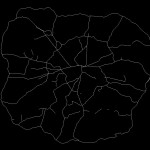
Top 2%
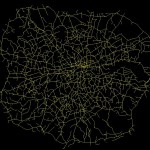
Top 5%
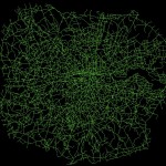
Top 10%
Top 20%
Defined A Roads and Motorways
The top 2% of these measures immediately draw out many of the most used and most well-known roads in London. The M25 is prominent, as is the North Circular and various corridor roads into the city. At 5% there is more definition of some of the other key roads, and by 10% we have a network that is quite similar to the map of ‘main’ roads in London.
By way of a statistically breakdown, the top 2% of values of the Choice measure predicts 76.3% of all ‘Motorway’ segments and 28.4% of all ‘A Roads’. By 10%, these values have risen to 87.4% and 75.4% of all segments, respectively. It is therefore clear that there is a correlation between this network measure and the definitions applied to the network.
I realise that this is a somewhat unrefined piece of work but I’d welcome any comments and am happy to share more on my method and results for those who are interested.
Looks like the MIT City Form Research Group have developed a very useful toolkit for those interested in small-scale urban network analysis. Bit uncertain about how well it might run on larger urban networks, if I get around to testing it I’ll put the results on here.