Something I have been thinking about recently is the possibility of integration between GIS and space syntax. The motivations are very clear. Space syntax represents a compelling quantitative model of human behaviour and movement. While the understanding of human systems is one of its most important areas of GIScience research (I may be slightly biased). And with the ever increasing availability of movement data on a range of levels, the development of a model underlying this behaviour is ever more important. So why can’t these two just get it on?
Representation
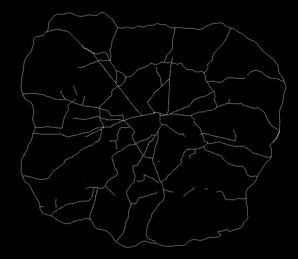
Well, the old argument has been that axial maps – the fundamental representation of space syntax – is simply not compatible with GIS. Axial lines represent lines of sight, while GIS data segments are supposedly geographically accurate – at the level of network measures this difference is highly significant. However, developments in space syntax – notably the development of Angular Segment Analysis by the brilliant Alasdair Turner, who very sadly died last week – mean that GIS integration is very much a possibility.
Turner’s approach was to measure the angular deviation between road segments on a GIS layer, assigning a score of zero for straight-ahead travel. The greater the movement away from the straight line the higher the score, effectively yielding a new axial line. Running angular betweenness (aka ‘choice’ in space syntax circles) calculations on the network yields some interesting results that I have discussed previously. The story is clearly much more complex than this (and more can be read on this here). But essentially this could be viewed as a new link between the traditional view of space syntax and GIScience.
ASA to the rescue?
However, some recent work I’ve been carrying out suggests that the picture is not so simple. Specifically, it is not necessarily possible to run an Angular Segment Analysis on a raw GIS layer. Taking the example of the OS ITN dataset – the most extensive representation of the UK road network – the presence of dual carriageways, roundabouts and other artefacts are contrary to what one would expect from an equivalent to the axial map. And, indeed, betweeness measures on these networks do not inspire either, with strange variations across the datasets, notably across dual carriageways where big discrepancies can be found.
There are two key aspects at play here, I feel. Firstly, ASA in it’s current form does not take account of traffic infrastructure and regulations. Were it to perhaps handle routing information then the results may be more realistic, certainly in terms of the flow on dual carriageways and roundabouts. Second, dual carriageways and roundabouts do not align with the fundamental idea behind the axial map. Cognitively speaking, we do not think in terms of dual carriageways, rather simply the existence of a roadway at a given location. In other words, why should dual carriageways be assessed independently since they were only simply engineered into two lanes?
Roadmap?
So, what can be the way forward here? Well, I know that where ASA is used commercially, the underlying network model is initially simplified to remove dual carriageways and roundabouts. But this seems awfully unscientific (well, maybe cartography isn’t particularly scientific either…). My suggestion, and something I am currently pursuing, is usage of simpler, existing GIS datasets. In this way, these models are already used widely and better validated than a subjective in-house alteration. Yet, what about other models and datasets that require more extensive GIS data? I suggest the development of tools that link together different GIS datasets, allowing an exchange of data yet not disrupting the validity of each approach. We can even try to link the axial map back to a range of GIS layers, and truly gain an understanding about the strengths of these approaches.
This is something I’ll be working on over the next few months – so watch this space, or get in touch if you’re interested in this.